Understanding the Levinson-Durbin Algorithm
Digital Signal Processing
Mathematics
I’ve recently been playing with this algorithm and wanted to do a write-up of my…
Building a digital filter for use in synthesisers
Digital Signal Processing
State Space Representation
Digital Filters
Synthesis
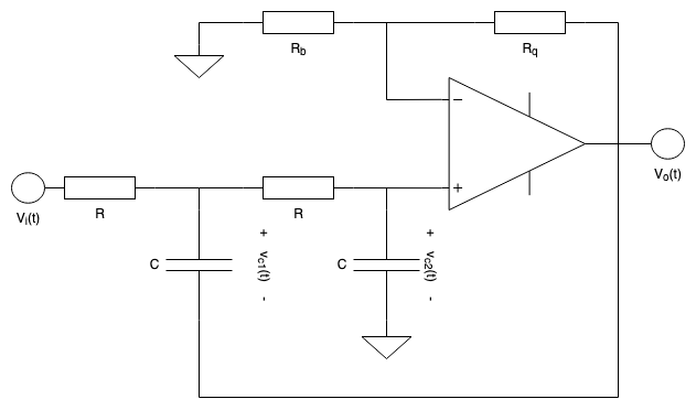
This is a tutorial on how to build a digital implementation of a 2nd-order, continuously-variable filter (i.e. one where you can change the parameters runtime) that has…
Even More Householder
Mathematics
Linear Algebra
Householder Matrix
In several previous blogs (here and here)…
An attempt at an intuitive description of the QR decomposition using Householder reflectors
Mathematics
Linear Algebra
Householder Matrix
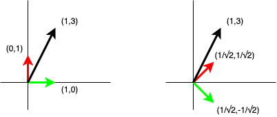
I really like the Householder matrix. I’ve blogged about its ability to generate an orthonormal basis containing a particular vector in a previous blog post. This blog post is a bit of a tutorial which will use the Householder matrix to perform a QR decomposition. Applying Householder reflectors to compute a QR decomposition is…
On the perils of cross-fading loops in organ samples
Digital Signal Processing
Crossfading
Sampled Pipe Organs
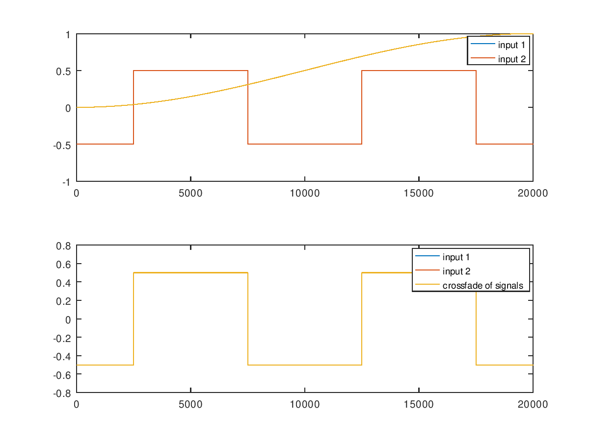
One common strategy when looping problematic organ samples is to employ a cross-fade. This is an irreversible audio modification that gradually transitions the samples…
Arbitrary polynomial-segment signal generation
Mathematics
State Space Representation
Digital Signal Processing
Synthesis
There is a tool which is part of my Open Diapason virtual organ project called “sampletune” which is designed to allow sample-set creators to tune samples by ear and save…
Three step digital Butterworth design
Digital Signal Processing
Digital Filters
This guide omits a fair amount of detail in order to provide a fairly quick guide.
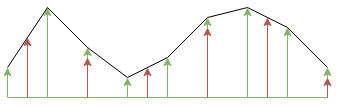
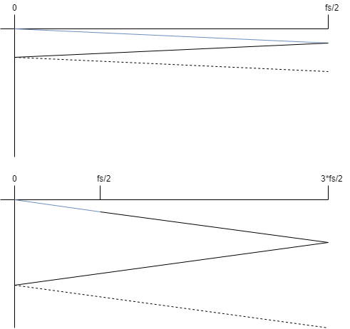
Real-time re-sampling and linear interpolation
Digital Signal Processing
Digital Filters
Multirate Signal Processing
Resampling
Disclaimer: I’ve intentionally tried to keep this post “non-mathy” - I want it to provide a…
Release alignment in sampled pipe organs – part 1
Digital Signal Processing
Sampled Pipe Organs
Crossfading
Correlation
A sample from a digital pipe organ contains at least:
Derivation of fast DCT-4 algorithm based on DFT
Mathematics
Discrete Cosine Transform
It’s well known that an \(N\) point DCT-4 can be computed using an \(N/2\) point complex FFT. Although the algorithm is widespread, the texts which I have read on the subject have not provided the details as to how it works. I’ve been trying to…
No matching items