I really like the Householder matrix. I’ve blogged about its ability to generate an orthonormal basis containing a particular vector in a previous blog post. This blog post is a bit of a tutorial which will use the Householder matrix to perform a QR decomposition. Applying Householder reflectors to compute a QR decomposition is nothing new, but I want this blog post to attempt to provide some intuition into how the algorithm works starting from almost nothing. We’ll briefly visit inner products, matrix multiplication, the Householder matrix and then build a QR decomposition in C. I’m not going to use formal language to define these operations unless it’s necessary. I’m going to assume that you understand things like matrix multiplication and what a matrix inverse is, but not much more than that. The post will be written assuming complex numbers are being used (the C implementation will not… maybe I will add one later).
The inner product
The inner product takes two vectors and produces a scalar. You can think of a vector as being an array of length \(N\) values representing coordinates in some N-dimensional space.
\[ \langle \mathbf{a}, \mathbf{b} \rangle = \sum^{N}_{k=1} a_k \overline{b_k} \]
Note the bar in the above indicates conjugation. If \(\mathbf{a}\) and \(\mathbf{b}\) are row vectors, we could write the above as:
\[ \langle \mathbf{a}, \mathbf{b} \rangle = \mathbf{a} \mathbf{b}^H \]
Where \(\mathbf{b}^H\) is the transposed conjugate of \(\mathbf{b}\) . Two vectors are said to be orthogonal if they have an inner product of zero. If the inner product of a vector with itself is equal to one, the vector is said to be a unit-vector. The inner product of a vector with a unit-vector is the proportion of that vector that is pointing in the same direction as the unit-vector i.e. if \(\mathbf{u}\) is some unit vector and I define a new vector as:
\[ \mathbf{b} = \mathbf{a} - \langle \mathbf{a}, \mathbf{u} \rangle \mathbf{u} \]
The vector \(\mathbf{b}\) is now orthogonal to \(\mathbf{u}\) i.e. \(\langle\mathbf{b},\mathbf{u}\rangle = 0\) .
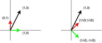
There are some good geometric visualisations of these for two and three dimensional vectors… but everything continues to work in arbitrary dimensions. The above image contains two plots which both contain two perpendicular unit vectors (red and green) and an arbitrary vector (black). In both plots we can verify the red and green vectors are unit vectors by applying the inner product. We can also verify they are orthogonal by applying the inner product. If we compute the inner product of the black vector on the two unit vectors, then multiply each of the scalar results by the corresponding unit vectors used to compute them and sum the results, we should get back the black vector.
Matrix multiplications
We can define matrix multiplication using inner products of the vectors which make up the rows of the left-hand side matrix with the vectors which make up the columns of the right-hand side matrix.
\[ \begin{pmatrix} \langle r_0, \overline{c_0} \rangle & \langle r_0, \overline{c_1} \rangle & \dots & \langle r_0, \overline{c_{N-1}} \rangle \\ \langle r_1, \overline{c_0} \rangle & \langle r_1, \overline{c_1} \rangle & \dots & \langle r_1, \overline{c_{N-1}} \rangle \\ \vdots & \vdots & & \vdots \\ \langle r_{M-1}, \overline{c_0} \rangle & \langle r_{M-1}, \overline{c_1} \rangle & \dots & \langle r_{M-1}, \overline{c_{N-1}} \rangle \end{pmatrix} = \begin{pmatrix} \dots & r_0 & \dots \\ \dots & r_1 & \dots \\ & \vdots & \\ \dots & r_{M-1} & \dots \end{pmatrix} \begin{pmatrix} \vdots & \vdots & & \vdots \\ c_0 & c_1 & \dots & c_{N-1} \\ \vdots & \vdots & & \vdots \end{pmatrix} \]
We can use this to demonstrate that a matrix that is made up of rows (or columns) that are all orthogonal to each other is trivially invertible - particularly if the vectors are unit vectors, in which case the inverse of matrix \(\mathbf{A}\) is \(\mathbf{A}^H\) . To make this particularly clear:
\[ \begin{pmatrix} \langle r_0, r_0 \rangle & \langle r_0, r_1 \rangle & \dots & \langle r_0, r_{N-1} \rangle \\ \langle r_1, r_0 \rangle & \langle r_1, r_1 \rangle & \dots & \langle r_1, r_{N-1} \rangle \\ \vdots & \vdots & & \vdots \\ \langle r_{N-1}, r_0 \rangle & \langle r_{N-1}, r_1 \rangle & \dots & \langle r_{N-1}, r_{N-1} \rangle \end{pmatrix} = \begin{pmatrix} \dots & r_0 & \dots \\ \dots & r_1 & \dots \\ & \vdots & \\ \dots & r_{N-1} & \dots \end{pmatrix} \begin{pmatrix} \vdots & \vdots & & \vdots \\ \overline{r_0} & \overline{r_1} & \dots & \overline{r_{N-1}} \\ \vdots & \vdots & & \vdots \end{pmatrix} \]
If the rows are orthogonal to each other, the inner products off the main diagonal will all be zero. If the rows are unit vectors, the diagonal entries are by definition \(1\) and \(\mathbf{I} = \mathbf{A}\mathbf{A}^H\) .
The Householder matrix
Define a matrix \(\mathbf{P}\) as:
\[\mathbf{P}=\mathbf{I} - 2\mathbf{v}\mathbf{v}^H\]
Where \(\mathbf{v}\) is a unit vector. Then:
\[\begin{array}{@{}ll@{}} \mathbf{P}\mathbf{P} &= \mathbf{I}-2\left(\mathbf{v}\mathbf{v}^H+\mathbf{v}\mathbf{v}^H\right)+4\mathbf{v}\mathbf{v}^H\mathbf{v}\mathbf{v}^H \\ &= \mathbf{I}-4\mathbf{v}\mathbf{v}^H+4\mathbf{v}\left(\mathbf{v}^H\mathbf{v}\right)\mathbf{v}^H \\ & = \mathbf{I} \end{array}\]
Thereore \(\mathbf{P}\) is its own inverse (\(\mathbf{P}=\mathbf{P}^{-1}\)) and must also be unitary (\(\mathbf{P}=\mathbf{P}^H\)).
If we can work out a method to choose \(\mathbf{v}\) such that \(\mathbf{P}\) will contain a particular unit vector \(\mathbf{u}\) and we multiply \(\mathbf{P}\) by any scaled version of vector \(\mathbf{u}\) , we will get a vector which has only one non-zero entry (because all other rows of the matrix will be orthogonal to \(\mathbf{u}\) ). I have described this process before in a previous blog post but will repeat it here with some more detail. Define a vector \(\mathbf{u}\) that we want the first column of \(\mathbf{P}\) to equal:
\[ \begin{array}{@{}ll@{}} \mathbf{u} &= \left( \mathbf{I} - 2 \mathbf{v} \mathbf{v}^H \right) \mathbf{e}_1 \\ \frac{\mathbf{e}_1-\mathbf{u}}{2} &= \mathbf{v} \overline{v_1} \end{array} \]
If \(u_1\) is real, we can break \(\mathbf{v}\) into its individual coordinates to solve for their values:
\[ \begin{array}{@{}ll@{}} v_1 &= \sqrt{\frac{1-u_1}{2}} \\ v_2 &= \frac{-u_2}{2\sqrt{\frac{1-u_1}{2}}} \\ &\vdots \\ v_n &= \frac{-u_n}{2\sqrt{\frac{1-u_1}{2}}} \end{array} \]
Given the way the matrix is defined, the computation of the square root is unnecessary in an implementation. This is best seen if we expand out the \(2\mathbf{v}\mathbf{v}^H\) matrix:
\[ \begin{array}{@{}ll@{}} 2 \mathbf{v} \mathbf{v}^H &= \begin{pmatrix} 2 v_1 \overline{v_1} & 2 v_1 \overline{v_2} & \dots & 2 v_1 \overline{v_n} \\ 2 v_2 \overline{v_1} & 2 v_2 \overline{v_2} & \dots & 2 v_2 \overline{v_n} \\ \vdots & \vdots & \ddots & \vdots \\ 2 v_n \overline{v_1} & 2 v_n \overline{v_2} & \dots & 2 v_n \overline{v_n} \end{pmatrix} \\ &= \begin{pmatrix} 1 - u_1 & -\overline{u_2} & \dots & -\overline{u_n} \\ -u_2 & \frac{u_2 \overline{u_2}}{1-u_1} & \dots & \frac{u_2 \overline{u_n}}{1-u_1} \\ \vdots & \vdots & \ddots & \vdots \\ -u_n & \frac{u_n \overline{u_2}}{1-u_1} & \dots & \frac{u_n \overline{u_n}}{1-u_1} \end{pmatrix} \end{array} \]
Define a scalar \(\alpha=\frac{1}{1-u_1}\) and a vector \(\mathbf{w}\) : \[\mathbf{w} = \begin{pmatrix}1 - u_1 \\ -u_2 \\ \vdots \\ -u_n \end{pmatrix} \]
Then \(2\mathbf{v}\mathbf{v}^H = \alpha \mathbf{w}\mathbf{w}^H\) . This is a particularly useful formulation because we rarely want to compute \(\mathbf{P}\) in its entirity and perform a matrix mutliplication. Rather, we compute:
\[ \mathbf{P}\mathbf{A} = \left(\mathbf{I}-\alpha\mathbf{w}\mathbf{w}^H\right)\mathbf{A}=\mathbf{A}-\alpha\mathbf{w}\mathbf{w}^H\mathbf{A} \]
Which is substantially more efficient. A final necessary change is necessary: if \(u_1\) is close to one (which implies all other coefficients of \(\mathbf{u}\) are approaching zero), \(\alpha\) will begin to approach infinity. There is a relatively simple change here which is to recognise that \(\mathbf{u}\) and \(-\mathbf{u}\) are parallel but pointing in different directions (their inner-product is \(-1\)). If we don’t care about the direction of the vector, we can change its sign to be the most numerically suitiable for the selection of \(\alpha\) i.e. if \(u_1 < 0\) use \(\mathbf{u}\) otherwise use \(-\mathbf{u}\).
This is actually very useful in many applications, one of which is the QR decomposition.
The QR decomposition
The QR decomposition breaks down a matrix \(\mathbf{A}\) into a unitary matrix \(\mathbf{Q}\) and an upper-triangular matrix \(\mathbf{R}\). There are a number of ways to do this, but we are going use the Householder matrix.
\[\mathbf{A} = \mathbf{Q}\mathbf{R}\]
Let’s start by defining a series of unitary transformations applied to \(\mathbf{A}\) as:
\[ \begin{array}{@{}ll@{}} \mathbf{X}_1&=\mathbf{P}_N \mathbf{A} \\ \mathbf{X}_{2} &= \begin{pmatrix} \mathbf{I}_{1} & \mathbf{0} \\ \mathbf{0} & \mathbf{P}_{N-1} \end{pmatrix} \mathbf{X}_{1} \\ \mathbf{X}_{3} &= \begin{pmatrix} \mathbf{I}_{2} & \mathbf{0} \\ \mathbf{0} & \mathbf{P}_{N-2} \end{pmatrix} \mathbf{X}_{2} \\ & \vdots \\ \mathbf{X}_{N-1} &= \begin{pmatrix} \mathbf{I}_{N-2} & \mathbf{0} \\ \mathbf{0} & \mathbf{P}_{2} \end{pmatrix} \mathbf{X}_{N-2} \end{array} \]
Where \(\mathbf{P}_n\) are all n-by-n unitary matrices. Notice that the first row of \(\mathbf{X}_1\) will be unmodified by all the transforms that follow. The first two rows of \(\mathbf{X}_2\) will be unmodified by all the transforms that follow - and so-on.
If we can somehow force the first row of \(\mathbf{P}_N\) to be the first column of \(\mathbf{A}\) scaled to be a unit vector (while keeping \(\mathbf{P}_N\) unitary), the first column of \(\mathbf{X}_1\) will contain only one non-zero entry. We then set about finding a way to select \(\mathbf{P}_{N-1}\) such that the second column contains only two non-zero entries… and so on. Once the process is finished, \(\mathbf{X}_{N-1}\) is upper triangular and the unitary matrix which converts \(\mathbf{A}\) into this form can be written as:
\[ \mathbf{Q}^H = \begin{pmatrix} \mathbf{I}_{N-2} & \mathbf{0} \\ \mathbf{0} & \mathbf{P}_{2} \end{pmatrix} \dots \begin{pmatrix} \mathbf{I}_{2} & \mathbf{0} \\ \mathbf{0} & \mathbf{P}_{N-2} \end{pmatrix} \begin{pmatrix} \mathbf{I}_{1} & \mathbf{0} \\ \mathbf{0} & \mathbf{P}_{N-1} \end{pmatrix} \mathbf{P}_N \]
And:
\[ \begin{array}{@{}ll@{}} \mathbf{X}_{N-1} &= \mathbf{Q}^H\mathbf{A} \\ \mathbf{Q}\mathbf{X}_{N-1}&=\mathbf{A} \end{array} \]
When we follow the above process and the \(\mathbf{P}_n\) matricies are chosen to be Householder matrices, we have performed the QR decomposition using Householder matrices.
Follows is the C code that implements the decomposition. Because the algorithm repeatedly applies transformations to \(\mathbf{A}\) to eventually arrive at \(\mathbf{R}\) , we will design an API that operates in-place on the supplied matrix. The orthogonal matrix will be built in parallel. The N-1 iterations over the i variable, correspond to the N-1 transformation steps presented earlier. I make no claims about the computational performance of this code. The numerical performance could be improved by using a different method to compute the length of the vector (first thing that happens in the column loop).
/* Perform the QR decomposition of the given square A matrix.
 * A/R is stored and written in columns i.e.
 * a[0] a[3] a[6]
 * a[1] a[4] a[7]
 * a[2] a[5] a[8]
 *
 * q is stored in rows i.e.
 * q[0] q[1] q[2]
 * q[3] q[4] q[5]
 * q[6] q[7] q[8] */
void qr(double *a_r, double *q, int N) {
    int i, j, k;

    /* Initialise qt to be the identity matrix. */
    for (i = 0; i < N; i++) {
        for (j = 0; j < N; j++) {
            q[i*N+j] = (i == j) ? 1.0 : 0.0;
        }
    }

    for (i = 0; i < N-1; i++) {
        double  norm, invnorm, alpha;
        double *ccol = a_r + i*N;

        /* Compute length of vector (needed to perform normalisation). */
        for (norm = 0.0, j = i; j < N; j++) {
            norm += ccol[j] * ccol[j];
        }
        norm = sqrt(norm);

        /* Flip the sign of the normalisation coefficient to have the
         * effect of negating the u vector. */
        if (ccol[0] > 0.0)
            norm = -norm;
        invnorm = 1.0 / norm;

        /* Normalise the column
         * Convert the column in-place into the w vector
         * Compute alpha */
        ccol[i] = (1.0 - ccol[i] * invnorm);
        for (j = i+1; j < N; j++) {
            ccol[j] = -ccol[j] * invnorm;
        }
        alpha = 1.0 / ccol[i];

        /* Update the orthogonal matrix */
        for (j = 0; j < N; j++) {
            double acc = 0.0;
            for (k = i; k < N; k++) {
                acc += ccol[k] * q[k+j*N];
            }
            acc *= alpha;
            for (k = i; k < N; k++) {
                q[k+j*N] -= ccol[k] * acc;
            }
        }

        /* Update the upper triangular matrix */
        for (j = i+1; j < N; j++) {
            double acc = 0.0;
            for (k = i; k < N; k++) {
                acc += ccol[k] * a_r[k+j*N];
            }
            acc *= alpha;
            for (k = i; k < N; k++) {
                a_r[k+j*N] -= ccol[k] * acc;
            }
        }

        /* Overwrite the w vector with the column data. */
        ccol[i] = norm;
        for (j = i+1; j < N; j++) {
            ccol[j] = 0.0;
        }
    }
}
The algorithm follows almost everthing described on this page - albiet with some minor obfuscations (the \(\mathbf{w}\) vector is stored temporarily in the output matrix to avoid needing any extra storage). It’s worth mentioning that the first step of initialising the \(\mathbf{Q}\) matrix to \(\mathbf{I}\) isn’t necessary. The initialisation could be performed explicitly in the first iteration of the loop over i - but that introduces more conditional code.