This is the first blog in what will probably be a series on the benefits of using state-space representation to implement discrete infinite impulse response (IIR) filters. Before I write about state-space and some of the things you can do with it, I want to give an overview of the difference equation and explain (hopefully intuitively) why they can be a poor choice for implementing a filter.
The discrete difference equation
The discrete difference equation takes an input value, a list of previous input values and a list of previous output values and combines them linearly to produce the next output value. This is codified mathematically in the following equation which can be recognised as the sum of two convolutions:
\[ y[n] = \sum_{k=0}^{N_b} b[k] x[n-k] - \sum_{k=1}^{N_a} a[k] y[n-k] \]
Instead of the above, we could write the difference equation as two distinct difference equations chained together:
\[ \begin{array}{@{}ll@{}} w[n] &= \sum_{k=0}^{N_b} b[k] x[n-k] \\ y[n] &= w[n] - \sum_{k=1}^{N_a} a[k] y[n-k] \end{array} \]
\(w[n]\) is the output of an all-zero filter which is used as input into an all-pole filter to produce \(y[n]\). If we were to take the z-transforms of the two filters, we would see quite plainly that we can also swap the order of the filters as:
\[ \begin{array}{@{}ll@{}} q[n] &= x[n] - \sum_{k=1}^{N_a} a[k] q[n-k] \\ y[n] &= \sum_{k=0}^{N_b} b[k] q[n-k] \end{array} \]
This time, \(q[n]\) is the output of an all-pole filter which is used as input into an all-zero filter to produce \(y[n]\). If we set \(N=N_a=N_b\), the benefit of this representation is that the two filters share exactly the same state and so an implementation needs not have delay lines for both output and input. This formulation has the name “Direct Form II” and is a popular implementation choice.
Regardless of whether we implement the difference equation directly or use Direct Form II, the implementation is easy to realise in a C program given a set of filter coefficients… so why would we want to do anything differently?
When difference equations go bad…
Let's build a 6-th order elliptic filter and run the difference equation explicitly using the following GNU Octave code. The filter is designed with a passband edge frequency of 240 Hz at a 48000 Hz sample rate (which isn't particularly low) with 6 dB of ripple in the passband and 80 dB of stopband attenuation.
N = 6;
IRLen = 8000;
[b, a] = ellip(N, 6, 80.0, 240.0/24000);
dp_y = zeros(IRLen, 1);
q = zeros(N, 1);
x = 1;
for i = 1:IRLen
qv = x - a(2:end) * q;
dp_y(i) = b * [qv; q];
q = [qv; q(1:(N-1))];
x = 0;
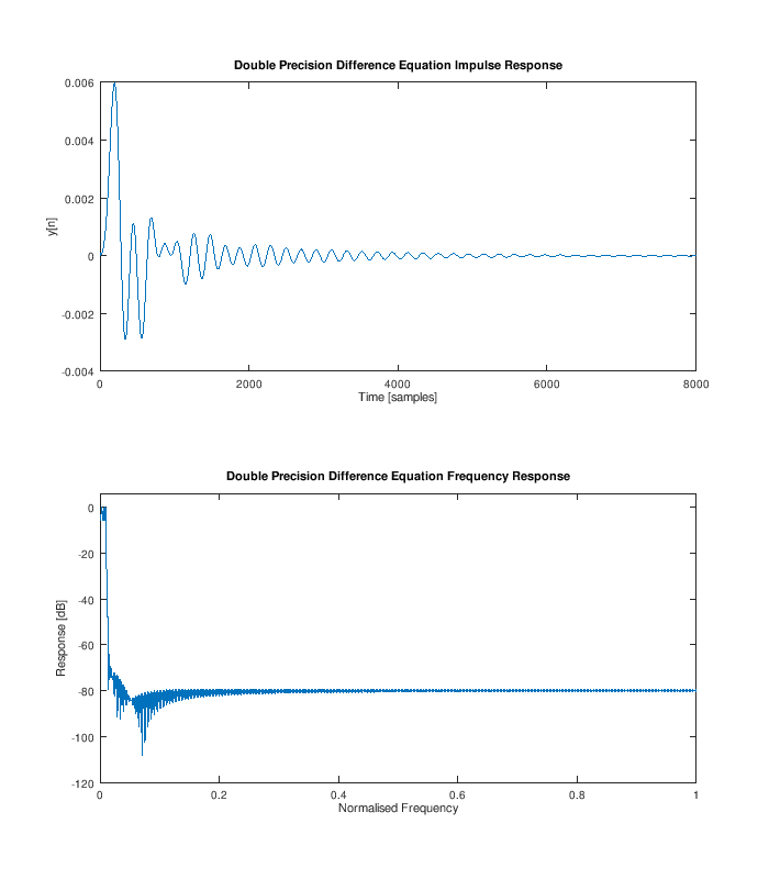
endAnd here is a plot of the impulse response and frequency response (which both look pretty good!):
Oh yeah, Octave by default is using double-precision for everything. Because we like fast things, let's specify that the states should always be stored using single precision by replacing the initialisation of q with:
q = single(zeros(N, 1));
And here is the new impulse response:
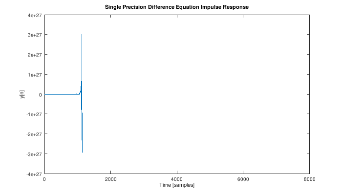
Bugger! Storing the states in single precision has lead to an instability in the filter. Small errors in the state are somehow being amplified by the coefficients of the difference equation and the output is growing without bound.
I'm going to try and give some intuition here: imagine that you are trying to synthesise a low-frequency discretely-sampled sinusoid that follows a slowly decaying exponential envelope. You've found that there is a z-transform that does exactly what you want from a z-transform table:
\[ a^n \sin(\omega_0 n) u[n] \Leftrightarrow \frac{a z \sin(\omega_0)}{z^2 - 2az\cos(\omega_0) + a^2} \]
You decide to implement the difference equation directly using Direct Form II leading to states that are the previous outputs of the impulse response of the all-pole component of the system.
The intuition is this: the values of the states close to \(t=0\) are all very close to zero - but after sufficient time, will eventually reach a very high-peak relative to their starting point without any external influence. Tiny errors in these small state values could grow by multiple orders of magnitude as the state evolves. This effectively happens at every zero crossing of the signal - and that is just illustrative component of the problem.
Ideally, the energy in the states of the system would only ever decrease when \(x[n]=0\) regardless of the values of \(y[n]\). Unfortunately, this almost never happens with a resonant system implemented using a difference equation. We should ask the question: can we find better states than previous outputs of the all-pole filter?
State-space
The Direct Form II difference equations presented earlier utilising \(q[n]\) and \(y[n]\) can be mutated into some fairly gross matrix equations:
\[ \begin{array}{@{}ll@{}} \begin{pmatrix} q[n-N+1] \\ \vdots \\ q[n-2] \\ q[n-1] \\ q[n] \end{pmatrix} &= \begin{pmatrix} 0 & 1 & 0 & \dots & 0 \\ 0 & \ddots & \ddots & \ddots & \vdots \\ 0 & \dots & 0 & 1 & 0 \\ 0 & \dots & 0 & 0 & 1 \\ -a[N] & \dots & -a[3] & -a[2] & -a[1] \end{pmatrix} \begin{pmatrix} q[n-N] \\ \vdots \\ q[n-3] \\ q[n-2] \\ q[n-1] \end{pmatrix} + \begin{pmatrix} 0 \\ \vdots \\ \vdots \\ 0 \\ 1 \end{pmatrix} x[n] \\ y[n] &= \begin{pmatrix} b[N]-a[N]b[0] & \dots & b[2]-a[2]b[0] & b[1]-a[1]b[0] \end{pmatrix} \begin{pmatrix} q[n-N] \\ \vdots \\ q[n-2] \\ q[n-1] \end{pmatrix} + b[0] x[n] \end{array} \]
Work through these and convince yourself they are equivalent. We can rewrite this entire system giving names to the matrices as:
\[ \begin{array}{@{}ll@{}} \mathbf{q}[n+1] &= \mathbf{A}\mathbf{q}[n] + \mathbf{B}\mathbf{x}[n] \\ \mathbf{y}[n] &= \mathbf{C} \mathbf{q}[n] + \mathbf{D}\mathbf{x}[n] \end{array} \]
These matrix equations are a state-space representation. The explicitly listed matrices before it are known as a “controllable canonical form” representation (for the case when \(b[0]=0\)). \(\mathbf{q}\) is the state vector and in controllable canonical form, it holds previous values of \(q[n]\) as described in the difference equations earlier.
So why would we want to do this? Who cares that we mapped a difference equation into a set of matrix equations? I'm going to list out some reasons which probably deserve their own blogs:
- Ability to analyse system using a vast array of matrix mathematical tools.
- Improve the numerical stability of the system.
- Preserving physical meanings of states during discretisation.
- Ability to design for efficient implementations.
In this blog, we're going to look at points one and two briefly to attempt to address the problems shown earlier.
Firstly, let's write the state equations in terms of their z-transforms so that we can build an expression that maps input to output:
\[ \begin{array}{@{}ll@{}} z\mathbf{Q}(z) &= \mathbf{A}\mathbf{Q}(z) + \mathbf{B}\mathbf{X}(z) \\ \mathbf{Y}(z) &= \mathbf{C} \mathbf{Q}(z) + \mathbf{D}\mathbf{X}(z) \end{array} \]
Doing some rearranging and substitution enables us to eliminate \(\mathbf{Q}(z)\):
\[\begin{array}{@{}ll@{}} z\mathbf{Q}(z) &= \mathbf{A}\mathbf{Q}(z)+\mathbf{B}\mathbf{X}(z) \\ \left(\mathbf{I}z-\mathbf{A}\right)\mathbf{Q}(z) &= \mathbf{B}\mathbf{X}(z) \\ \mathbf{Q}(z) &= \left(\mathbf{I}z-\mathbf{A}\right)^{-1} \mathbf{B}\mathbf{X}(z) \\ \mathbf{Y}(z) &= \left( \mathbf{C}\left(\mathbf{I}z-\mathbf{A}\right)^{-1} \mathbf{B}+\mathbf{D} \right) \mathbf{X}(z) \\ &= \frac{\mathbf{C}\text{ adj}\left(\mathbf{I}z-\mathbf{A}\right) \mathbf{B}+\mathbf{D}\det\left(\mathbf{I}z-\mathbf{A}\right) }{\det\left(\mathbf{I}z-\mathbf{A}\right)} \mathbf{X}(z) \end{array}\]
The \(\det\left(\mathbf{I}z-\mathbf{A}\right)\) term in the denominator expands to the characteristic polynomial of \(\mathbf{A}\) in \(z\) and if we are trying to map a z-domain transfer function to a state-space system, it needs to equal the denominator of the transfer function. Just as the poles of a transfer function are roots of the denominator, the poles of a state-space system are the eigenvalues of the \(\mathbf{A}\) matrix. The numerator of the above expression is a matrix of polynomials in \(z\) showing how state-space is naturally able to handle multiple-input multiple-output (MIMO) systems.
Earlier, we asked can we pick better values for the states? Before getting to that, let's answer a different question: can we pick different values for the states? The answer is: yes - and we can prove it trivially by substituting \(\mathbf{q}[n]\) with \(\mathbf{W}^{-1}\hat{\mathbf{q}}[n]\) where \(\mathbf{W}\) is some invertible square matrix:
\[ \begin{array}{@{}ll@{}} \mathbf{W}^{-1}\hat{\mathbf{q}}[n+1] &= \mathbf{A}\mathbf{W}^{-1}\hat{\mathbf{q}}[n] + \mathbf{B}\mathbf{x}[n] \\ \hat{\mathbf{q}}[n+1] &= \mathbf{W}\mathbf{A}\mathbf{W}^{-1}\hat{\mathbf{q}}[n] + \mathbf{W}\mathbf{B}\mathbf{x}[n] \\ \mathbf{y}[n] &= \mathbf{C} \mathbf{W}^{-1}\hat{\mathbf{q}}[n] + \mathbf{D}\mathbf{x}[n] \end{array} \]
This changes the coordinate system that the state vector exists in. We can pick any invertible matrix \(\mathbf{W}\) and use it to modify a system's \(\mathbf{A}\), \(\mathbf{B}\) and \(\mathbf{C}\) matrices keeping the system output \(\mathbf{y}[n]\) identical. The quantity \(\mathbf{W}\mathbf{A}\mathbf{W}^{-1}\) is a similarity transform on \(\mathbf{A}\) and it preserves the eigenvalues/characteristic polynomial of \(\mathbf{A}\) for all invertible \(\mathbf{W}\).
State-space degrees of freedom
The coefficients of a difference equation are unique for a particular impulse response. The coefficients of the state-space representation for \(N>1\) are not. In-fact, we have already demonstrated this previously by showing we can change the coordinate system of the state-vector.
Let's go through the process of taking a 2x2 SISO system and finding the transfer function.
\[ \begin{array}{@{}ll@{}} \frac{Y(z)}{X(z)} &= \frac{\mathbf{C}\text{ adj}\left(\mathbf{I}z-\mathbf{A}\right) \mathbf{B}+\mathbf{D}\det\left(\mathbf{I}z-\mathbf{A}\right) }{\det\left(\mathbf{I}z-\mathbf{A}\right)} \\ &= \frac{\begin{pmatrix}c_0 & c_1\end{pmatrix}\text{ adj}\begin{pmatrix}z-a_{00} & -a_{01} \\ -a_{10} & z-a_{11}\end{pmatrix} \begin{pmatrix}b_0 \\ b_1\end{pmatrix}+d\det\begin{pmatrix}z-a_{00} & -a_{01} \\ -a_{10} & z-a_{11}\end{pmatrix} }{\det\begin{pmatrix}z-a_{00} & -a_{01} \\ -a_{10} & z-a_{11}\end{pmatrix}} \\ &= \frac{\begin{pmatrix}c_0 & c_1\end{pmatrix}\begin{pmatrix}z-a_{11} & a_{01} \\ a_{10} & z-a_{00}\end{pmatrix} \begin{pmatrix}b_0 \\ b_1\end{pmatrix}+d\left((z-a_{00})(z-a_{11})-a_{01}a_{10}\right)}{(z-a_{00})(z-a_{11})-a_{01}a_{10}} \\ &= \frac{c_0(b_0(z-a_{11}) + b_1a_{01}) + c_1(b_0a_{10} + b_1(z-a_{00}))+d\left((z-a_{00})(z-a_{11})-a_{01}a_{10}\right)}{(z-a_{00})(z-a_{11})-a_{01}a_{10}} \\ &= \frac{dz^2+z(c_0b_0+c_1b_1-d(a_{00}+a_{11}))+c_0(b_1a_{01}-b_0a_{11})+c_1(b_0a_{10}-b_1a_{00})+d(a_{00}a_{11}-a_{01}a_{10})}{z^2-z(a_{00}+a_{11}) + a_{00}a_{11}-a_{01}a_{10}} \end{array} \]
We can select all of these quantities to match a given second order transfer function - but how should we choose them? What makes for good coefficients? What does good mean? We could force some values to zero or one to minimize multiplies? If we want to improve numeric performance, given that the \(\mathbf{A}\) matrix is responsible for moving states forward in time, it seems reasonable to minimize the impact that errors in the state vector can have when multiplied by \(\mathbf{A}\) - this is akin to making \(\mathbf{A}\) as well conditioned as possible. This might be a good strategy for fixing our example 6th order system.
Orthogonal matrices are well-conditioned and for those deeply familiar with IIR design, you may also know that the state update for a coupled form IIR implementation is effectively determined by an orthonormal matrix that has been attenuated by some scalar. Coupled form state-updates can only be used to mimic a conjugate pole pair, but for every classical IIR design (Butterworth, Chebyshev I/II, Cauer/Elliptic) of even order (like our example 6th order problematic system), all the poles are in conjugate pairs. Start by defining \(\mathbf{A}\) as an orthogonal matrix:
\[ \mathbf{A} = \begin{pmatrix}a_{00} & -a_{10} \\ a_{10} & a_{00} \end{pmatrix} \]
The transfer function becomes:
\[ \frac{Y(z)}{X(z)} = \frac{dz^2+z(c_0b_0+c_1b_1-2da_{00})+c_0(-b_1a_{10}-b_0a_{00})+c_1(b_0a_{10}-b_1a_{00})+d(a_{00}^2+a_{10}^2)}{z^2-2za_{00} + a_{00}^2+a_{10}^2} \]
There are two remaining free variables we can pick. Somewhat arbitrarily, we will select \(c_0=1\) and \(c_1=0\) to get:
\[ \frac{Y(z)}{X(z)} = \frac{dz^2+z(b_0-2da_{00})-b_1a_{10}-b_0a_{00}+d(a_{00}^2+a_{10}^2)}{z^2-2za_{00} + a_{00}^2+a_{10}^2} \]
We now have a system of equations we can solve for the unknown matrix quantities that will create a state-space system that mimics a 2nd order resonant transfer function.
Chaining systems together
Consider we have two systems which we would like to connect together:
\[ \begin{array}{@{}ll@{}} z\mathbf{Q}_1(z) &= \mathbf{A}_1\mathbf{Q}_1(z) + \mathbf{B}_1\mathbf{X}(z) \\ \mathbf{U}(z) &= \mathbf{C}_1 \mathbf{Q}_1(z) + \mathbf{D}_1\mathbf{X}(z) \end{array} \]
And:
\[ \begin{array}{@{}ll@{}} z\mathbf{Q}_2(z) &= \mathbf{A}_2\mathbf{Q}_2(z) + \mathbf{B}_2\mathbf{U}(z) \\ \mathbf{Y}(z) &= \mathbf{C}_2 \mathbf{Q}_2(z) + \mathbf{D}_2\mathbf{U}(z) \end{array} \]
We can make direct substitutions to get:
\[ \begin{array}{@{}ll@{}} z\mathbf{Q}_1(z) &= \mathbf{A}_1\mathbf{Q}_1(z) + \mathbf{B}_1\mathbf{X}(z) \\ z\mathbf{Q}_2(z) &= \mathbf{A}_2\mathbf{Q}_2(z) + \mathbf{B}_2\mathbf{C}_1 \mathbf{Q}_1(z) + \mathbf{B}_2 \mathbf{D}_1\mathbf{X}(z) \\ \mathbf{Y}(z) &= \mathbf{C}_2 \mathbf{Q}_2(z) + \mathbf{D}_2\mathbf{C}_1 \mathbf{Q}_1(z) + \mathbf{D}_2\mathbf{D}_1\mathbf{X}(z) \end{array} \]
We can re-write the above as a set of block matrix equations:
\[ \begin{array}{@{}ll@{}} z\begin{pmatrix}\mathbf{Q}_2(z) \\ \mathbf{Q}_1(z)\end{pmatrix} &= \begin{pmatrix} \mathbf{A}_2 & \mathbf{B}_2 \mathbf{C}_1 \\ \mathbf{0} & \mathbf{A}_1 \end{pmatrix} \begin{pmatrix}\mathbf{Q}_2(z) \\ \mathbf{Q}_1(z)\end{pmatrix} + \begin{pmatrix}\mathbf{B}_2 \mathbf{D}_1 \\ \mathbf{B}_1\end{pmatrix} \mathbf{X}(z) \\ \mathbf{Y}(z) &= \begin{pmatrix}\mathbf{C}_2 & \mathbf{D}_2 \mathbf{C}_1 \end{pmatrix}\begin{pmatrix}\mathbf{Q}_2(z) \\ \mathbf{Q}_1(z)\end{pmatrix} + \mathbf{D}_2 \mathbf{D}_1 \mathbf{X}(z) \end{array} \]
This provides a direct method for connecting systems together into one larger system. As \(\mathbf{A}\) is an upper-triangular block-diagonal matrix, the eigenvalues of the new system are the same as those of the existing systems and the \(\mathbf{B}_2\mathbf{C}_1\) term in the connected system has no influence. Given that, can we decouple the sections completely? i.e. can we completely eliminate the \(\mathbf{B}_2\mathbf{C}_1\) term by using a similarity transform as described previously? Let's pose the question using block matrices:
\[ \begin{pmatrix} \mathbf{A}_2 & \mathbf{0} \\ \mathbf{0} & \mathbf{A}_1 \end{pmatrix} \begin{pmatrix} \mathbf{W}_{00} & \mathbf{W}_{01} \\ \mathbf{W}_{10} & \mathbf{W}_{11} \end{pmatrix} = \begin{pmatrix} \mathbf{W}_{00} & \mathbf{W}_{01} \\ \mathbf{W}_{10} & \mathbf{W}_{11} \end{pmatrix} \begin{pmatrix} \mathbf{A}_2 & \mathbf{B}_2 \mathbf{C}_1 \\ \mathbf{0} & \mathbf{A}_1 \end{pmatrix} \]
\[ \begin{array}{@{}ll@{}} \mathbf{A}_2 \mathbf{W}_{00} &= \mathbf{W}_{00} \mathbf{A}_2 \\ \mathbf{A}_1 \mathbf{W}_{10} &= \mathbf{W}_{10} \mathbf{A}_2 \\ \mathbf{A}_2 \mathbf{W}_{01} &= \mathbf{W}_{00} \mathbf{B}_2 \mathbf{C}_1 + \mathbf{W}_{01} \mathbf{A}_1 \\ \mathbf{A}_1 \mathbf{W}_{11} &= \mathbf{W}_{10} \mathbf{B}_2 \mathbf{C}_1 + \mathbf{W}_{11} \mathbf{A}_1 \end{array} \]
There is only one valid set of solutions for these equations:
\[ \begin{array}{@{}ll@{}} \mathbf{W}_{00} &= \mathbf{I} \\ \mathbf{W}_{11} &= \mathbf{I} \\ \mathbf{W}_{10} &= \mathbf{0} \\ \mathbf{A}_2 \mathbf{W}_{01} - \mathbf{W}_{01} \mathbf{A}_1 &= \mathbf{B}_2 \mathbf{C}_1 \end{array} \]
Where the final equation is a Sylvester equation which can be solved without too much pain programatically (i.e. using a matrix inverse) if and only if \(\mathbf{A}_1\) and \(\mathbf{A}_2\) share no common eigenvalues. If we do this, we end up with the following system:
\[ \begin{array}{@{}ll@{}} z\begin{pmatrix}\mathbf{Q}_2(z) \\ \mathbf{Q}_1(z)\end{pmatrix} &= \begin{pmatrix} \mathbf{A}_2 & \mathbf{0} \\ \mathbf{0} & \mathbf{A}_1 \end{pmatrix} \begin{pmatrix}\mathbf{Q}_2(z) \\ \mathbf{Q}_1(z)\end{pmatrix} + \mathbf{W}\begin{pmatrix}\mathbf{B}_2 \mathbf{D}_1 \\ \mathbf{B}_1\end{pmatrix} \mathbf{X}(z) \\ \mathbf{Y}(z) &= \begin{pmatrix}\mathbf{C}_2 & \mathbf{D}_2 \mathbf{C}_1 \end{pmatrix}\mathbf{W}^{-1}\begin{pmatrix}\mathbf{Q}_2(z) \\ \mathbf{Q}_1(z)\end{pmatrix} + \mathbf{D}_2 \mathbf{D}_1 \mathbf{X}(z) \end{array} \]
This will be better conditioned and have some other benefits in terms of efficient implementations. This block-diagonalisation we just performed is the equivalent of performing the partial-fraction decomposition on the cascaded system (which I've never seen a nice looking algorithmic solution for).
Bringing it home
Let's take our problematic 6th order system, break it up into 3 second order state-space sections using the coupled-form mapping we described and evaluate the performace again:
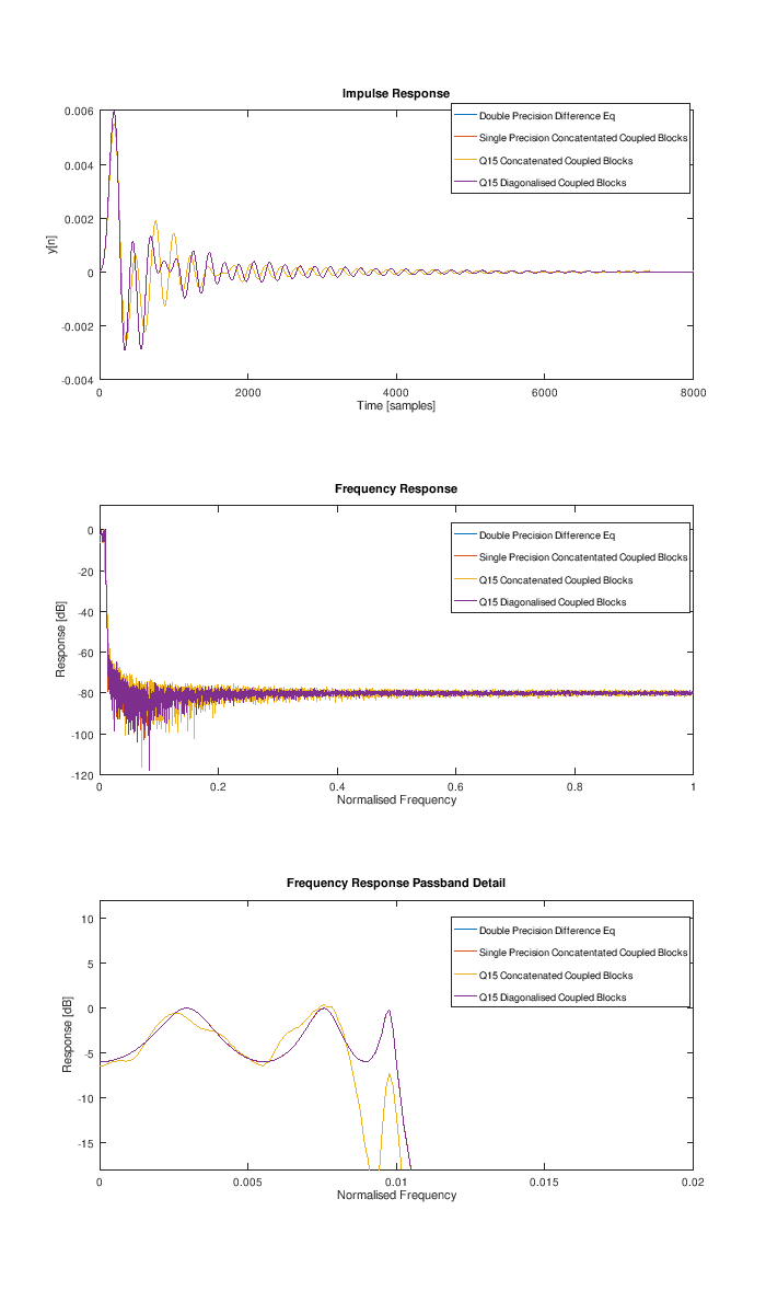
There are 4 data-sets:
- The original double-precision difference equation results.
- The concatenated coupled-form systems without block-diagonalisation storing the states in single precision.
- The concatenated coupled-form systems without block-diagonalisation storing the states in a q15 format (15 bits of fractional precision).
- The concatenated coupled-form systems with block-diagonalisation storing the states in q15 format.
The performance difference between 2 and the block-diagonalised system with states in signle precision is negligible and so is not included in the plots. The performance difference between 1, 2 and 4 is practiacally identical in the passband. There is some fudging going on with the q15 plots because the precision is fixed but the range is not. I've tried to make things more even by:
- 2-Norm matching the \(\mathbf{B}\) and \(\mathbf{C}\) matrices of the systems without diagonalisation.
- 2-Norm matching each sub-section of the \(\mathbf{B}\) and \(\mathbf{C}\) matrices of the system with diagonalisation (which we can do because they are all operating independetly).
- 2-Norm matching the \(\mathbf{C}\) matrices of the diagonalised and undiagonalised systems after the above has happened (which also requires modifying \(\mathbf{B}\)).
The performance of 1, 2 and 4 are all incredibly good. The performance of 3 shows that cascading leads to error build-up that significantly compromises the output.
These coupled-form state-space filter realisations are good down to very low frequencies. I have had success synthesising sub 10 Hz 16th order elliptic filters that work just fine with single-precision floating point. Next time, we'll look at preservation of state meanings when we discretise an analogue system.